Announcing RStudio v1.0!

Today we’re very pleased to announce the availability of RStudio Version 1.0! Version 1.0 is our 10th major release since the initial launch in February 2011 (see the full release history below), and our biggest ever! Highlights include:

• Authoring tools for R Notebooks.
• Integrated support for the sparklyr package (R interface to Spark).
• Performance profiling via integration with the profvis package.
• Enhanced data import tools based on the readr, readxl and haven packages.
• Authoring tools for R Markdown websites and the bookdown package.
• Many other miscellaneous enhancements and bug fixes.

We hope you download version 1.0 now and as always let us know what you think.

R Notebooks

R Notebooks add a powerful notebook authoring engine to R Markdown. Notebook interfaces for data analysis have compelling advantages including the close association of code and output and the ability to intersperse narrative with computation. Notebooks are also an excellent tool for teaching and a convenient way to share analyses.

Interactive R Markdown

As an authoring format, R Markdown bears many similarities to traditional notebooks like Jupyter and Beaker. However, code in notebooks is typically executed interactively, one cell at a time, whereas code in R Markdown documents is typically executed in batch.

R Notebooks bring the interactive model of execution to your R Markdown documents, giving you the capability to work quickly and iteratively in a notebook interface without leaving behind the plain-text tools, compatibility with version control, and production-quality output you’ve come to rely on from R Markdown.

Iterate Quickly

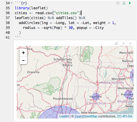
In a typical R Markdown document, you must re-knit the document to see your changes, which can take some time if it contains non-trivial computations. R Notebooks, however, let you run code and see the results in the document immediately. They can include just about any kind of content R produces, including console output, plots, data frames, and interactive HTML widgets.

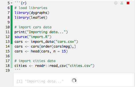
You can see the progress of the code as it runs:

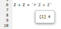
You can preview the results of individual inline expressions, too:

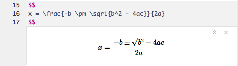
Even your LaTeX equations render in real-time as you type:

This focused mode of interaction doesn’t require you to keep the console, viewer, or output panes open. Everything you need is at your fingertips in the editor, reducing distractions and helping you concentrate on your analysis. When you’re done, you’ll have a formatted, reproducible record of what you’ve accomplished, with plenty of context, perfect for your own records or sharing with others.

Spark with sparklyr

The sparklyr package is a new R interface for Apache Spark. RStudio now includes integrated support for Spark and the sparklyr package, including tools for:

• Creating and managing Spark connections
• Browsing the tables and columns of Spark DataFrames
• Previewing the first 1,000 rows of Spark DataFrames

Once you’ve installed the sparklyr package, you should find a new Spark pane within the IDE. This pane includes a New Connection dialog which can be used to make connections to local or remote Spark instances:

Once you’ve connected to Spark you’ll be able to browse the tables contained within the Spark cluster:

The Spark DataFrame preview uses the standard RStudio data viewer:

Profiling with profvis

“How can I make my code faster?”

If you write R code, then you’ve probably asked yourself this question. A profiler is an important tool for doing this: it records how the computer spends its time, and once you know that, you can focus on the slow parts to make them faster.

RStudio now includes integrated support for profiling R code and for visualizing profiling data. R itself has long had a built-in profiler, and now it’s easier than ever to use the profiler and interpret the results.

To profile code with RStudio, select it in the editor, and then click on Profile -> Profile Selected Line(s). R will run that code with the profiler turned on, and then open up an interactive visualization.

In the visualization, there are two main parts: on top, there is the code with information about the amount of time spent executing each line, and on the bottom there is a flame graph, which shows what R was doing over time. In the flame graph, the horizontal direction represents time, moving from left to right, and the vertical direction represents the call stack, which are the functions that are currently being called. (Each time a function calls another function, it goes on top of the stack, and when a function exits, it is removed from the stack.)

The Data tab contains a call tree, showing which function calls are most expensive:

Armed with this information, you’ll know what parts of your code to focus on to speed things up!

Data Import

RStudio now integrates with the readr, readxl, and haven packages to provide comprehensive tools for importing data from many text file formats, Excel worksheets, as well as SAS, Stata, and SPSS data files. The tools are focused on interactively refining an import then providing the code required to reproduce the import on new datasets.

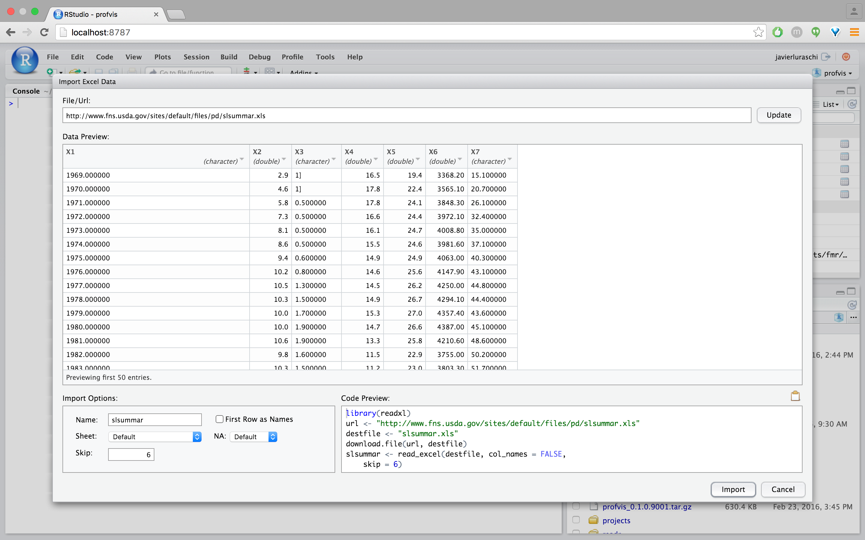
For example, here’s the workflow we would use to import the Excel worksheet at http://www.fns.usda.gov/sites/default/files/pd/slsummar.xls.

First provide the dataset URL and review the import in preview mode (notice that this file contains two tables and as a result requires the first few rows to be removed):

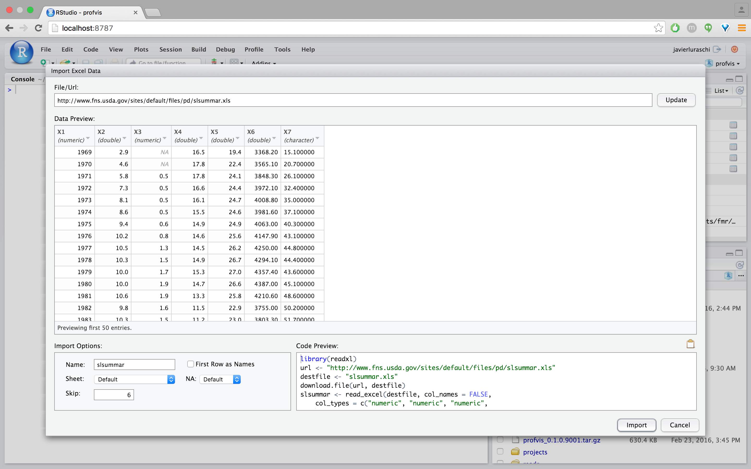
We can clean this up by skipping 6 rows from this file and unchecking the “First Row as Names” checkbox:

The file is looking better but some columns are being displayed as strings when they are clearly numerical data. We can fix this by selecting “numeric” from the column drop-down:

The final step is to click “Import” to run the code displayed under “Code Preview” and import the data into R. The code is executed within the console and imported dataset is displayed automatically:

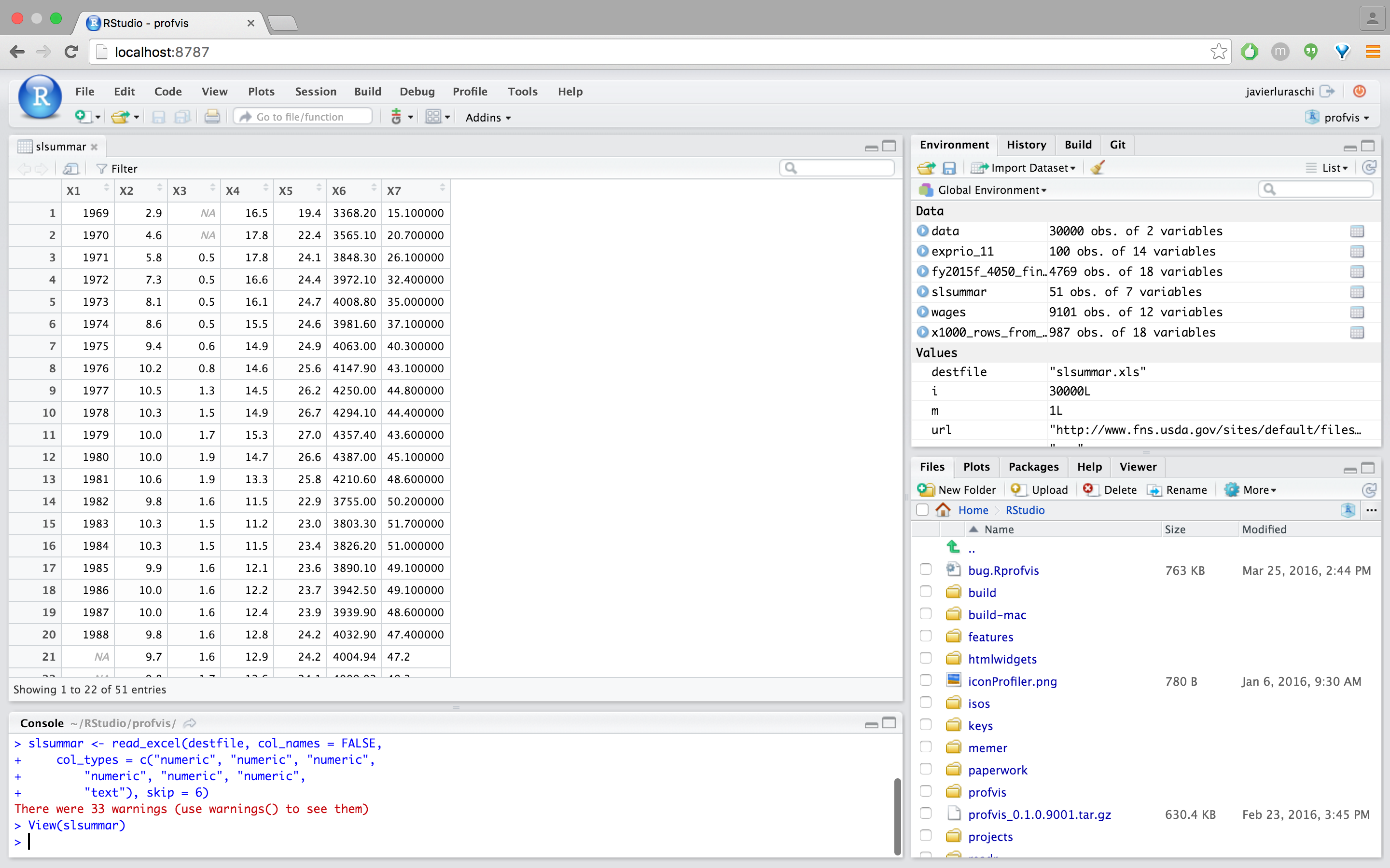
Note that rather than executing the import we could have just copied and pasted the import code and included it within any R script.

RStudio Release History

We started working on RStudio in November of 2008 (8 years ago!) and had our first public release in February of 2011. Here are highlights of the various releases through the years:

Version	Date	Highlights
0.92	Feb 2011	Initial public release
0.93	Apr 2011	Interactive plotting with manipulate Source editor themes Configurable workspace layout
0.94	Jun 2011	Enhanced plot export Enhanced package installation and management Enhanced history management
0.95	Jan 2012	RStudio project system Code navigation (typeahead search, go to definition) Version control integration (Git and Subversion)
0.96	May 2012	Enhanced authoring for Sweave Web publishing with R Markdown Code folding and many other editing enhancements
0.97	Oct 2012	Package development tools Vim editing mode More intelligent R auto-indentation
0.98	Dec 2013	Interactive debugging tools Enhanced environment pane Viewer pane for web content / htmlwidgets
0.98b	Jun 2014	R Markdown v2 (publish to PDF, Word, and more) Integrated tools for Shiny application development Editor support for XML, SQL, Python, and Bash
0.99	May 2015	Data viewer with support for large datasets, filtering, searching, and sorting Major enhancements to R and C/C++ code completion and inline code diagnostics Multiple cursors, tab re-ordering, enhanced Vim mode
0.99b	Feb 2016	Emacs editing mode Multi-window source editing Customizable keyboard shortcuts RStudio Addins
1.0	Nov 2016	Authoring tools for R Notebooks Integrated support for sparklyr (R interface to Spark) Enhanced data import tools Performance profiling via integration with profvis

The RStudio Release History page on our support website provides a complete history of all major and minor point releases.

 

sparklyr — R interface for Apache Spark

We’re excited today to announce sparklyr, a new package that provides an interface between R and Apache Spark.

Over the past couple of years we’ve heard time and time again that people want a native dplyr interface to Spark, so we built one! sparklyr also provides interfaces to Spark’s distributed machine learning algorithms and much more. Highlights include:

• Interactively manipulate Spark data using both dplyr and SQL (via DBI).
• Filter and aggregate Spark datasets then bring them into R for analysis and visualization.
• Orchestrate distributed machine learning from R using either Spark MLlib or H2O SparkingWater.
• Create extensions that call the full Spark API and provide interfaces to Spark packages.
• Integrated support for establishing Spark connections and browsing Spark data frames within the RStudio IDE.

We’re also excited to be working with several industry partners. IBM is incorporating sparklyr into their Data Science Experience, Cloudera is working with us to ensure that sparklyr meets the requirements of their enterprise customers, and H2O has provided an integration between sparklyr and H2O Sparkling Water.

Getting Started

You can install sparklyr from CRAN as follows:

install.packages("sparklyr")

You should also install a local version of Spark for development purposes:

library(sparklyr)
spark_install(version = "1.6.2")

If you use the RStudio IDE, you should also download the latest preview release of the IDE which includes several enhancements for interacting with Spark.

Extensive documentation and examples are available at http://spark.rstudio.com.

Connecting to Spark

You can connect to both local instances of Spark as well as remote Spark clusters. Here we’ll connect to a local instance of Spark:

library(sparklyr)
sc <- spark_connect(master = "local")

The returned Spark connection (sc) provides a remote dplyr data source to the Spark cluster.

Reading Data

You can copy R data frames into Spark using the dplyr copy_to function (more typically though you’ll read data within the Spark cluster using the spark_read family of functions). For the examples below we’ll copy some datasets from R into Spark (note that you may need to install the nycflights13 and Lahman packages in order to execute this code):

library(dplyr)
iris_tbl <- copy_to(sc, iris)
flights_tbl <- copy_to(sc, nycflights13::flights, "flights")
batting_tbl <- copy_to(sc, Lahman::Batting, "batting")

Using dplyr

We can now use all of the available dplyr verbs against the tables within the cluster. Here’s a simple filtering example:

# filter by departure delay
flights_tbl %>% filter(dep_delay == 2)

Introduction to dplyr provides additional dplyr examples you can try. For example, consider the last example from the tutorial which plots data on flight delays:

delay <- flights_tbl %>% 
  group_by(tailnum) %>%
  summarise(count = n(), dist = mean(distance), delay = mean(arr_delay)) %>%
  filter(count > 20, dist < 2000, !is.na(delay)) %>%
  collect()

# plot delays
library(ggplot2)
ggplot(delay, aes(dist, delay)) +
  geom_point(aes(size = count), alpha = 1/2) +
  geom_smooth() +
  scale_size_area(max_size = 2)

Note that while the dplyr functions shown above look identical to the ones you use with R data frames, with sparklyr they use Spark as their back end and execute remotely in the cluster.

Window Functions

dplyr window functions are also supported, for example:

batting_tbl %>%
  select(playerID, yearID, teamID, G, AB:H) %>%
  arrange(playerID, yearID, teamID) %>%
  group_by(playerID) %>%
  filter(min_rank(desc(H)) <= 2 & H > 0)

For additional documentation on using dplyr with Spark see the dplyr section of the sparklyr website.

Using SQL

It’s also possible to execute SQL queries directly against tables within a Spark cluster. The spark_connection object implements a DBI interface for Spark, so you can use dbGetQuery to execute SQL and return the result as an R data frame:

library(DBI)
iris_preview <- dbGetQuery(sc, "SELECT * FROM iris LIMIT 10")

Machine Learning

You can orchestrate machine learning algorithms in a Spark cluster via either Spark MLlib or via the H2O Sparkling Water extension package. Both provide a set of high-level APIs built on top of DataFrames that help you create and tune machine learning workflows.

Spark MLlib

In this example we’ll use ml_linear_regression to fit a linear regression model. We’ll use the built-in mtcars dataset, and see if we can predict a car’s fuel consumption (mpg) based on its weight (wt) and the number of cylinders the engine contains (cyl). We’ll assume in each case that the relationship between mpg and each of our features is linear.

# copy mtcars into spark
mtcars_tbl <- copy_to(sc, mtcars)

# transform our data set, and then partition into 'training', 'test'
partitions <- mtcars_tbl %>%
  filter(hp >= 100) %>%
  mutate(cyl8 = cyl == 8) %>%
  sdf_partition(training = 0.5, test = 0.5, seed = 1099)

# fit a linear model to the training dataset
fit <- partitions$training %>%
  ml_linear_regression(response = "mpg", features = c("wt", "cyl"))

For linear regression models produced by Spark, we can use summary() to learn a bit more about the quality of our fit, and the statistical significance of each of our predictors.

summary(fit)

Spark machine learning supports a wide array of algorithms and feature transformations, and as illustrated above it’s easy to chain these functions together with dplyr pipelines. To learn more see the Spark MLlib section of the sparklyr website.

H2O Sparkling Water

Let’s walk the same mtcars example, but in this case use H2O’s machine learning algorithms via the H2O Sparkling Water extension. The dplyr code used to prepare the data is the same, but after partitioning into test and training data we call h2o.glm rather than ml_linear_regression:

# convert to h20_frame (uses the same underlying rdd)
training <- as_h2o_frame(partitions$training)
test <- as_h2o_frame(partitions$test)

# fit a linear model to the training dataset
fit <- h2o.glm(x = c("wt", "cyl"),
               y = "mpg",
               training_frame = training,
               lamda_search = TRUE)

# inspect the model
print(fit)

For linear regression models produced by H2O, we can use either print() or summary() to learn a bit more about the quality of our fit. The summary() method returns some extra information about scoring history and variable importance.

To learn more see the H2O Sparkling Water section of the sparklyr website.

Extensions

The facilities used internally by sparklyr for its dplyr and machine learning interfaces are available to extension packages. Since Spark is a general purpose cluster computing system there are many potential applications for extensions (e.g. interfaces to custom machine learning pipelines, interfaces to 3rd party Spark packages, etc.).

The sas7bdat extension enables parallel reading of SAS datasets in the sas7bdat format into Spark data frames. The rsparkling extension provides a bridge between sparklyr and H2O’s Sparkling Water.

We’re excited to see what other sparklyr extensions the R community creates. To learn more see the Extensions section of the sparklyr website.

RStudio IDE

The latest RStudio Preview Release of the RStudio IDE includes integrated support for Spark and the sparklyr package, including tools for:

• Creating and managing Spark connections
• Browsing the tables and columns of Spark DataFrames
• Previewing the first 1,000 rows of Spark DataFrames

Once you’ve installed the sparklyr package, you should find a new Spark pane within the IDE. This pane includes a New Connection dialog which can be used to make connections to local or remote Spark instances:

Once you’ve connected to Spark you’ll be able to browse the tables contained within the Spark cluster:

The Spark DataFrame preview uses the standard RStudio data viewer:

The RStudio IDE features for sparklyr are available now as part of the RStudio Preview Release. The final version of RStudio IDE that includes integrated support for sparklyr will ship within the next few weeks.

Partners

We’re very pleased to be joined in this announcement by IBM, Cloudera, and H2O, who are working with us to ensure that sparklyr meets the requirements of enterprise customers and is easy to integrate with current and future deployments of Spark.

IBM

“With our latest contributions to Apache Spark and the release of sparklyr, we continue to emphasize R as a primary data science language within the Spark community. Additionally, we are making plans to include sparklyr in Data Science Experience to provide the tools data scientists are comfortable with to help them bring business-changing insights to their companies faster,” said Ritika Gunnar, vice president of Offering Management, IBM Analytics.

Cloudera

“At Cloudera, data science is one of the most popular use cases we see for Apache Spark as a core part of the Apache Hadoop ecosystem, yet the lack of a compelling R experience has limited data scientists’ access to available data and compute,” said Charles Zedlewski, vice president, Products at Cloudera. “We are excited to partner with RStudio to help bring sparklyr to the enterprise, so that data scientists and IT teams alike can get more value from their existing skills and infrastructure, all with the security, governance, and management our customers expect.”

H2O

“At H2O.ai, we’ve been focused on bringing the best of breed open source machine learning to data scientists working in R & Python. However, the lack of robust tooling in the R ecosystem for interfacing with Apache Spark has made it difficult for the R community to take advantage of the distributed data processing capabilities of Apache Spark.

We’re excited to work with RStudio to bring the ease of use of dplyr and the distributed machine learning algorithms from H2O’s Sparkling Water to the R community via the sparklyr & rsparkling packages”

flexdashboard: Easy interactive dashboards for R

Today we’re excited to announce flexdashboard, a new package that enables you to easily create flexible, attractive, interactive dashboards with R. Authoring and customization of dashboards is done using R Markdown and you can optionally include Shiny components for additional interactivity.

Highlights of the flexdashboard package include:

• Support for a wide variety of components including interactive htmlwidgets; base, lattice, and grid graphics; tabular data; gauges; and value boxes.
• Flexible and easy to specify row and column-based layouts. Components are intelligently re-sized to fill the browser and adapted for display on mobile devices.
• Extensive support for text annotations to include assumptions, contextual narrative, and analysis within dashboards.
• Storyboard layouts for presenting sequences of visualizations and related commentary.
• By default dashboards are standard HTML documents that can be deployed on any web server or even attached to an email message. You can optionally add Shiny components for additional interactivity and then deploy on Shiny Server or shinyapps.io.

Getting Started

The flexdashboard package is available on CRAN; you can install it as follows:

install.packages("flexdashboard", type = "source")

To author a flexdashboard you create an R Markdown document with the flexdashboard::flex_dashboard output format. You can do this from within RStudio using the New R Markdown dialog:

Dashboards are simple R Markdown documents where each level 3 header (###) defines a section of the dashboard. For example, here’s a simple dashboard layout with 3 charts arranged top to bottom:

---
title: "My Dashboard"
output: flexdashboard::flex_dashboard
---

### Chart 1
 
```{r}

```
 
### Chart 2

```{r}

```

### Chart 3

```{r}

```

You can use level 2 headers (-----------) to introduce rows and columns into your dashboard and section attributes to control their relative size:

---
title: "My Dashboard"
output: flexdashboard::flex_dashboard
---

Column {data-width=600}
-------------------------------------
 
### Chart 1
 
```{r}

```
 
Column {data-width=400}
-------------------------------------
 
### Chart 2

```{r}

``` 
 
### Chart 3
 
```{r}

```

Learning More

The flexdashboard website includes extensive documentation on building your own dashboards, including:

• A user guide for all of the features and options of flexdashboard, including layout orientations (row vs. column based), chart sizing, the various supported components, theming, and creating dashboards with multiple pages.
• Details on using Shiny to create dashboards that enable viewers to change underlying parameters and see the results immediately, or that update themselves incrementally as their underlying data changes.
• A variety of sample layouts which you can use as a starting point for your own dashboards.
• Many examples of flexdashboard in action (including links to source code if you want to dig into how each example was created).

The examples below illustrate the use of flexdashboard with various packages and layouts (click the thumbnail to view a running version of each dashboard):

d3heatmap: NBA scoring

ggplotly: ggplot2 geoms

Shiny: biclust example

dygraphs: linked time series

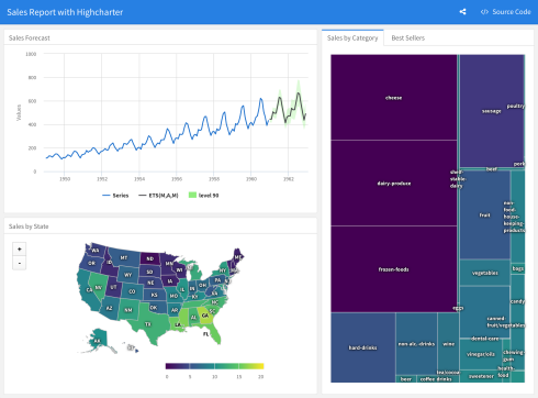
highcharter: sales report

Storyboard: htmlwidgets showcase

rbokeh: iris dataset

Shiny: diamonds explorer

 

Try It Out

The flexdashboard package provides a simple yet powerful framework for creating dashboards from R. If you know R Markdown you already know enough to begin creating dashboards right now! We hope you’ll try it out and let us know how it’s working and what else we can do to make it better.

 

R Markdown Custom Formats

The R Markdown package ships with a raft of output formats including HTML, PDF, MS Word, R package vignettes, as well as Beamer and HTML5 presentations. This isn’t the entire universe of available formats though (far from it!). R Markdown formats are fully extensible and as a result there are several R packages that provide additional formats. In this post we wanted to highlight a few of these packages, including:

• tufte — Documents in the style of Edward Tufte
• rticles — Formats for creating LaTeX based journal articles
• rmdformats — Formats for creating HTML documents

We’ll also discuss how to create your own custom formats as well as re-usable document templates for existing formats.

Using Custom Formats

Custom R Markdown formats are just R functions which return a definition of the format’s behavior. For example, here’s the metadata for a document that uses the html_document format:

---
title: "My Document"
output: html_document
---

When rendering, R Markdown calls the rmarkdown::html_document function to get the definition of the output format. A custom format works just the same way but is also qualified with the name of the package that contains it. For example, here’s the metadata for a document that uses the tufte_handout format:

---
title: "My Document"
output: tufte::tufte_handout
---

Custom formats also typically register a template that helps you get started with using them. If you are using RStudio you can easily create a new document based on a custom format via the New R Markdown dialog:

Tufte Handouts

The tufte package includes custom formats for creating documents in the style that Edward Tufte uses in his books and handouts. Tufte’s style is known for its extensive use of sidenotes, tight integration of graphics with text, and well-set typography. Formats for both LaTeX and HTML/CSS output are provided (these are in turn based on the work in tufte-latex and tufte-css). Here’s some example output from the LaTeX format:

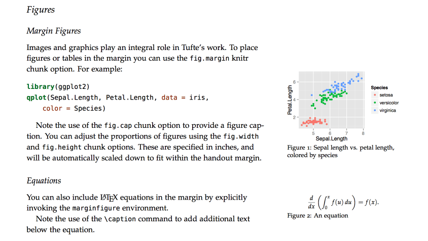
If you want LaTeX/PDF output, you can use the tufte_handout format for handouts and tufte_book for books. For HTML output, you use the tufte_html format. For example:

---
title: "An Example Using the Tufte Style"
author: "John Smith"
output:
  tufte::tufte_handout: default
  tufte::tufte_html: default
---

You can install the tufte package from CRAN as follows:

install.packages("tufte")

See the tufte package website for additional documentation on using the Tufte custom formats.

Journal Articles

The rticles package provides a suite of custom R Markdown LaTeX formats and templates for various journal article formats, including:

• JSS articles
• R Journal articles
• CTeX documents
• ACM articles
• ACS articles
• Elsevier journal submissions.

You can install the rticles package from CRAN as follows:

install.packages("rticles")

See the rticles repository for more details on using the formats included with the package. The source code of the rticles package is an excellent resource for learning how to create LaTeX based custom formats.

rmdformats Package

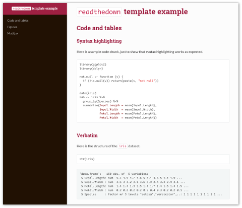
The rmdformats package from Julien Barnier includes three HTML based document formats that provide nice alternatives to the default html_document format that is included in the rmarkdown package. The readthedown format is inspired by the Read the docs Sphinx theme and is fully responsive, with collapsible navigation:

The html_docco and html_clean formats both provide provide automatic thumbnails for figures with lightbox display, and html_clean provides an automatic and dynamic table of contents:

 

You can install the rmdformats package from CRAN as follows:

install.packages("rmdformats")

See the rmdformats repository for documentation on using the readthedown, html_docco, and html_clean formats.

Creating New Formats

Hopefully checking out some of the custom formats described above has you inspired to create your very own new formats. The R Markdown website includes documentation on how to create a custom format. In addition, the source code of the tufte, rticles, and rmdformats packages provide good examples to work from.

Short of creating a brand new format, it’s also possible to create a re-usable document template that shows up within the RStudio New R Markdown dialog box. This would be appropriate if an existing template met your needs but you wanted to have an easy way to create documents with a pre-set list of options and skeletal content. See the article on document templates for additional details on how to do this.

R Markdown v0.9.5

A new release of the rmarkdown package is now available on CRAN. This release features some long-requested enhancements to the HTML document format, including:

1. The ability to have a floating (i.e. always visible) table of contents.
2. Folding and unfolding for R code (to easily show and hide code for either an entire document or for individual chunks).
3. Support for presenting content within tabbed sections (e.g. several plots could each have their own tab).
4. Five new themes including “lumen”, “paper”, “sandstone”, “simplex”, & “yeti”.

There are also three new formats for creating GitHub, OpenDocument, and RTF documents as well as a number of smaller enhancements and bug fixes (see the package NEWS for all of the details).

Floating TOC

You can specify the toc_float option to float the table of contents to the left of the main document content. The floating table of contents will always be visible even when the document is scrolled. For example:

---
title: "Habits"
output:
  html_document:
    toc: true
    toc_float: true
---

Here’s what the floating table of contents looks like on one of the R Markdown website’s pages:

Code Folding

When the knitr chunk option echo = TRUE is specified (the default behavior) the R source code within chunks is included within the rendered document. In some cases it may be appropriate to exclude code entirely (echo = FALSE) but in other cases you might want the code available but not visible by default.

The code_folding: hide option enables you to include R code but have it hidden by default. Users can then choose to show hidden R code chunks either indvidually or document wide. For example:

---
title: "Habits"
output:
  html_document:
    code_folding: hide
---

Here’s the default HTML document template with code folding enabled. Note that each chunk has it’s own toggle for showing or hiding code and there is also a global menu for operating on all chunks at once.

Note that you can specify code_folding: show to still show all R code by default but then allow users to hide the code if they wish.

Tabbed Sections

You can organize content using tabs by applying the .tabset class attribute to headers within a document. This will cause all sub-headers of the header with the .tabset attribute to appear within tabs rather than as standalone sections. For example:

## Sales Report {.tabset}

### By Product

(tab content)

### By Region

(tab content)

Here’s what tabbed sections look like within a rendered document:

Authoring Enhancements

We also shouldn’t fail to mention that the most recent release of RStudio included several enhancements to R Markdown document editing. There’s now an optional outline view that enables quick navigation across larger documents:

We also also added inline UI to code chunks for running individual chunks, running all previous chunks, and specifying various commonly used knit options:

What’s Next

We’ve got lots of additional work planned for R Markdown including new document formats, additional authoring enhancements in RStudio, and some new tools to make it easier to publish and manage documents created with R Markdown. More details to follow soon!

 

New Release of RStudio (v0.99.878)

We’re pleased to announce that a new release of RStudio (v0.99.878) is available for download now. Highlights of this release include:

• Support for registering custom RStudio Addins.
• R Markdown editing improvements including outline view and inline UI for chunk execution.
• Support for multiple source windows (tear editor tabs off main window).
• Pane zooming for working distraction free within a single pane.
• Editor and IDE keyboard shortcuts can now be customized.
• New Emacs keybindings mode for the source editor.
• Support for parameterized R Markdown reports.
• Various improvements to RStudio Server Pro including multiple concurrent R sessions, use of multiple R versions, and shared projects for collaboration.

There are lots of other small improvements across the product, check out the release notes for full details.

RStudio Addins

RStudio Addins provide a mechanism for executing custom R functions interactively from within the RStudio IDE—either through keyboard shortcuts, or through the Addins menu. Coupled with the rstudioapi package, users can now write R code to interact with and modify the contents of documents open in RStudio.

An addin can be as simple as a function that inserts a commonly used snippet of text, and as complex as a Shiny application that accepts input from the user and uses it to transform the contents of the active editor. The sky is the limit!

Here’s an example of addin that enables interactive subsetting of a data frame with live preview:

 

This addin is implemented using a Shiny Gadget (see the source code for more details). RStudio Addins are distributed as R packages. Once you’ve installed an R package that contains addins, they’ll be immediately become available within RStudio.

You can learn more about using and developing addins here: http://rstudio.github.io/rstudioaddins/.

R Markdown

We’ve made a number of improvements to R Markdown authoring. There’s now an optional outline view that enables quick navigation across larger documents:

We’ve also added inline UI to code chunks for running individual chunks, running all previous chunks, and specifying various commonly used knit options:

Multiple Source Windows

There are two ways to open a new source window:

Pop out an editor: click the Show in New Window button in any source editor tab.

Tear off a pane: drag a tab out of the main window and onto the desktop; a new source window will be opened where you dropped the tab.

You can have as many source windows open as you like. Each source window has its own set of tabs; these tabs are independent of the tabs in RStudio’s main source pane.

Customizable Keyboard Shortcuts

You can now customize keyboard shortcuts in RStudio — you can bind keys to execute RStudio application commands, editor commands, or even user-defined R functions.

Access the keyboard shortcuts by clicking Tools -> Modify Keyboard Shortcuts...:

This will present a dialog that enables remapping of all available editor commands (commands that affect the current document’s contents, or the current selection) and RStudio commands (commands whose actions are scoped beyond just the current editor).

Emacs Keybindings

We’ve introduced a new keybindings mode to go along with the default bindings and Vim bindings already supported. Emacs mode provides a base set of keybindings for navigation and selection, including:

• C-p, C-n, C-b and C-f to move the cursor up, down left and right by characters
• M-b, M-f to move left and right by words
• C-a, C-e to navigate to the start, or end, of line;
• C-k to ‘kill’ to end of line, and C-y to ‘yank’ the last kill,
• C-s, C-r to initiate an Emacs-style incremental search (forward / reverse),
• C-Space to set/unset mark, and C-w to kill the marked region.

There are some additional keybindings that Emacs Speaks Statistics (ESS) users might find familiar:

• C-c C-v displays help for the object under the cursor,
• C-c C-n evaluates the current line / selection,
• C-x b allows you to visit another file,
• M-C-a moves the cursor to the beginning of the current function,
• M-C-e moves to the end of the current function,
• C-c C-f evaluates the current function.

We’ve also introduced a number of keybindings that allow you to interact with the IDE as you might normally do in Emacs:

• C-x C-n to create a new document,
• C-x C-f to find / open an existing document,
• C-x C-s to save the current document,
• C-x k to close the current file.

RStudio Server Pro

We’ve introduced a number of significant enhancements to RStudio Server Pro in this release, including:

• The ability to open multiple concurrent R sessions. Multiple concurrent sessions are useful for running multiple analyses in parallel and for switching between different tasks.
• Flexible use of multiple R versions on the same server. This is useful when you have some analysts or projects that require older versions of R or R packages and some that require newer versions.

• Project sharing for easy collaboration within workgroups. When you share a project, RStudio Server securely grants other users access to the project, and when multiple users are active in the project at once, you can see each others’ activity and work together in a shared editor.

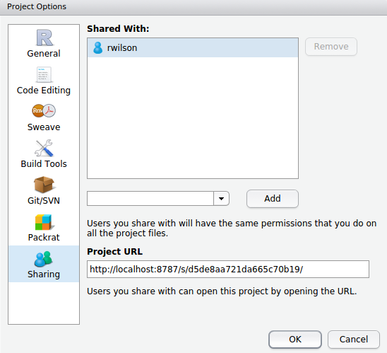
See the updated RStudio Server Pro page for additional details, including a set of videos which demonstrate the new features.

Try it Out

RStudio v0.99.878 is available for download now. We hope you enjoy the new release and as always please let us know how it’s working and what else we can do to make the product better.

 

 

RcppParallel: Getting R and C++ to work (some more) in parallel

(Post by Dirk Eddelbuettel and JJ Allaire)

A common theme over the last few decades was that we could afford to simply sit back and let computer (hardware) engineers take care of increases in computing speed thanks to Moore’s law. That same line of thought now frequently points out that we are getting closer and closer to the physical limits of what Moore’s law can do for us.

So the new best hope is (and has been) parallel processing. Even our smartphones have multiple cores, and most if not all retail PCs now possess two, four or more cores. Real computers, aka somewhat decent servers, can be had with 24, 32 or more cores as well, and all that is before we even consider GPU coprocessors or other upcoming changes.

Sometimes our tasks are embarrassingly simple as is the case with many data-parallel jobs: we can use higher-level operations such as those offered by the base R package parallel to spawn multiple processing tasks and gather the results. Dirk covered all this in some detail in previous talks on High Performance Computing with R (and you can also consult the CRAN Task View on High Performance Computing with R).

But sometimes we cannot use data-parallel approaches. Hence we have to redo our algorithms. Which is really hard. R itself has been relying on the (fairly mature) OpenMP standard for some of its operations. Luke Tierney’s keynote at the 2014 R/Finance conference mentioned some of the issues related to OpenMP, which works really well on Linux but currently not so well on other platforms. R is expected to make wider use of it in future versions once compiler support for OpenMP on Windows and OS X improves.

In the meantime, the RcppParallel package provides a complete toolkit for creating portable, high-performance parallel algorithms without requiring direct manipulation of operating system threads. RcppParallel includes:

• Intel Thread Building Blocks (v4.3), a C++ library for task parallelism with a wide variety of parallel algorithms and data structures (Windows, OS X, Linux, and Solaris x86 only).
• TinyThread, a C++ library for portable use of operating system threads.
• RVector and RMatrix wrapper classes for safe and convenient access to R data structures in a multi-threaded environment.
• High level parallel functions (parallelFor and parallelReduce) that use Intel TBB as a back-end on systems that support it and TinyThread on other platforms.

RcppParallel is available on CRAN now and several packages including dbmss, gaston, markovchain, rPref, SpatPCA, StMoSim, and text2vec are already taking advantage of it (you can read more about the tex2vec implementation here).

For more background and documentation see the RcppParallel web site as well as the slides from the talk we gave on RcppParallel at the Workshop for Distributed Computing in R.

In addition, the Rcpp Gallery includes several pieces demonstrating the use of RcppParallel, including:

• A parallel matrix transformation
• A parallel vector summation
• A parallel inner product
• A parallel distance matrix calculation

All four are interesting and demonstrate different aspects of parallel computing via RcppParallel. But the last article is key—it shows how a particular matrix distance metric (which is missing from R) can be implemented in a serial manner in both R, and also via Rcpp. The fastest implementation, however, uses both Rcpp and RcppParallel and thereby achieves a truly impressive speed gain as the gains from using compiled code (via Rcpp) and from using a parallel algorithm (via RcppParallel) are multiplicative. On a couple of four-core machines the RcppParallel version was between 200 and 300 times faster than the R version.

Exciting times for parallel programming in R! To learn more head over to the RcppParallel package and start playing.

Secure HTTPS Connections for R

Traditionally, the mechanisms for obtaining R and related software have used standard HTTP connections. This isn’t ideal though, as without a secure (HTTPS) connection there is less assurance that you are downloading code from a legitimate source rather than from another server posing as one.

Recently there have been a number of changes that make it easier to use HTTPS for installing R, RStudio, and packages from CRAN:

1. Downloads of R from the main CRAN website now use HTTPS;

2. Downloads of RStudio from our website now use HTTPS; and

3. It is now possible to install packages from CRAN over HTTPS.

There are a number of ways to ensure that installation of packages from CRAN are performed using HTTPS. The most recent version of R  (v3.2.2) makes this the default behavior. The most recent version of RStudio (v0.99.473) also attempts to configure secure downloads from CRAN by default (even for older versions of R). Finally, any version of R or RStudio can use secure HTTPS downloads by making some configuration changes as described in the Secure Package Downloads for R article in our Knowledge Base.

Configuring Secure Connections to CRAN

While the simplest way to ensure secure connections to CRAN is to run the updated versions mentioned above, it’s important to note that it is not necessary to upgrade R or RStudio to achieve this end. Rather, two configuration changes can be made:

1. The R download.file.method option needs to specify a method that is capable of HTTPS; and
2. The CRAN mirror you are using must be capable of HTTPS connections (not all of them are).

The specifics of the required changes for various products, platforms, and versions of R are described in-depth in the Secure Package Downloads for R article in our Knowledge Base.

Recommendations for RStudio Users

We’ve made several changes to RStudio IDE to ensure that HTTPS connections are used throughout the product:

1. The default download.file.method option is set to an HTTPS compatible method (with a warning displayed if a secure method can’t be set);
2. The configured CRAN mirror is tested for HTTPS compatibility and a warning is displayed if the mirror doesn’t support HTTPS;
3. HTTPS is used for user selection of a non-default CRAN mirror;
4. HTTPS is used for in-product documentation links;
5. HTTPS is used when checking for updated versions of RStudio (applies to desktop version only); and
6. HTTPS is used when downloading Rtools (applies to desktop version only).

If you are running RStudio on the desktop we strongly recommend that you update to the latest version (v0.99.473).

Recommendations for Server Administrators

If you are running RStudio Server it’s possible to make the most important security enhancements by changing your configuration rather than updating to a new version. The Secure Package Downloads for R article in our Knowledge Base provides documentation on how do this.

In this case in-product documentation links and user selection of a non-default CRAN mirror will continue to use HTTP rather than HTTPS however these are less pressing concerns than CRAN package installation. If you’d like these functions to also be performed over HTTPS then you should upgrade your server to the latest version of RStudio.

If you are running Shiny Server we recommend that you modify your configuration to support HTTPS package downloads as described in the Secure Package Downloads for R article.

Accelerating R: RStudio and the new R Consortium

To paraphrase Yogi Berra, “Predicting is hard, especially about the future”. In 1993, when Ross Ihaka and Robert Gentleman first started working on R, who would have predicted that it would be used by millions in a world that increasingly rewards data literacy? It’s impossible to know where R will go in the next 20 years, but at RStudio we’re working hard to make sure the future is bright.

Today, we’re excited to announce our participation in the R Consortium, a new 501(c)6 nonprofit organization. The R Consortium is a collaboration between the R Foundation, RStudio, Microsoft, TIBCO, Google, Oracle, HP and others. It’s chartered to fund and inspire ideas that will enable R to become an even better platform for science, research, and industry. The R Consortium complements the R Foundation by providing a convenient funding vehicle for the many commercial beneficiaries of R to give back to the community, and will provide the resources to embark on ambitious new projects to make R even better.

We believe the R Consortium is critically important to the future of R and despite our small size, we chose to join it at the highest contributor level (alongside Microsoft). Open source is a key component of our mission and giving back to the community is extremely important to us.

The community of R users and developers have a big stake in the language and its long-term success. We all want free and open source R to continue thriving and growing for the next 20 years and beyond. The fact that so many of the technology industry’s largest companies are willing to stand behind R as part of the consortium is remarkable and we think bodes incredibly well for the future of R.

New Version of RStudio (v0.99) Available Now

We’re pleased to announce that the final version of RStudio v0.99 is available for download now. Highlights of the release include:

• A new data viewer with support for large datasets, filtering, searching, and sorting.
• Complete overhaul of R code completion with many new features and capabilities.
• The source editor now provides code diagnostics (errors, warnings, etc.) as you work.
• User customizable code snippets for automating common editing tasks.
• Tools for Rcpp: completion, diagnostics, code navigation, find usages, and automatic indentation.
• Many additional source editor improvements including multiple cursors, tab re-ordering, and several new themes.
• An enhanced Vim mode with visual block selection, macros, marks, and subset of : commands.

There are also lots of smaller improvements and bug fixes across the product. Check out the v0.99 release notes for details on all of the changes.

Data Viewer

We’ve completely overhauled the data viewer with many new capabilities including live update, sorting and filtering, full text searching, and no row limit on viewed datasets.

See the data viewer documentation for more details.

Code Completion

Previously RStudio only completed variables that already existed in the global environment. Now completion is done based on source code analysis so is provided even for objects that haven’t been fully evaluated:

Completions are also provided for a wide variety of specialized contexts including dimension names in [ and [[:

Code Diagnostics

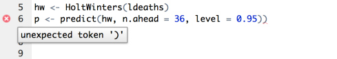
We’ve added a new inline code diagnostics feature that highlights various issues in your R code as you edit.

For example, here we’re getting a diagnostic that notes that there is an extra parentheses:

Here the diagnostic indicates that we’ve forgotten a comma within a shiny UI definition:

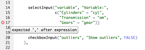
A wide variety of diagnostics are supported, including optional diagnostics for code style issues (e.g. the inclusion of unnecessary whitespace). Diagnostics are also available for several other languages including C/C++, JavaScript, HTML, and CSS. See the code diagnostics documentation for additional details.

Code Snippets

Code snippets are text macros that are used for quickly inserting common snippets of code. For example, the fun snippet inserts an R function definition:

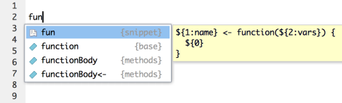
If you select the snippet from the completion list it will be inserted along with several text placeholders which you can fill in by typing and then pressing Tab to advance to the next placeholder:

Other useful snippets include:

• lib, req, and source for the library, require, and source functions
• df and mat for defining data frames and matrices
• if, el, and ei for conditional expressions
• apply, lapply, sapply, etc. for the apply family of functions
• sc, sm, and sg for defining S4 classes/methods.

See the code snippets documentation for additional details.

Try it Out

RStudio v0.99 is available for download now. We hope you enjoy the new release and as always please let us know how it’s working and what else we can do to make the product better.